1. Five decades of wolf-moose dynamics
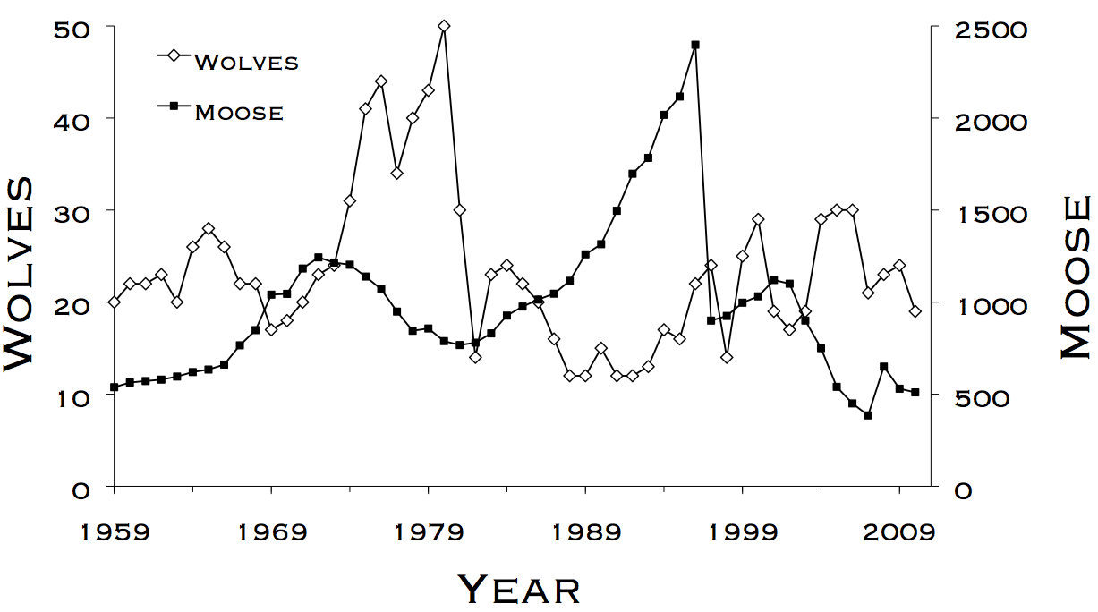
The wolves and moose of Isle Royale have been studied for more than five decades. This research represents the longest continuous study of any predator-prey system in the world.
The most important events in the chronology have been essentially unpredictable. In 1980 the wolf population crashed when humans inadvertently introduced a disease, canine-parvovirus. In 1996, the moose population collapsed during the most severe winter on record and an unexpected outbreak of moose ticks. In the late 1990s, intense levels of inbreeding among wolves were mitigated when a wolf immigrated from Canada. In response, the wolf population generally increased throughout the early 21st century, despite declining moose abundance. For a more detailed interpretation of this graph, click here.
2. How are wolf and moose abundances related to one another?
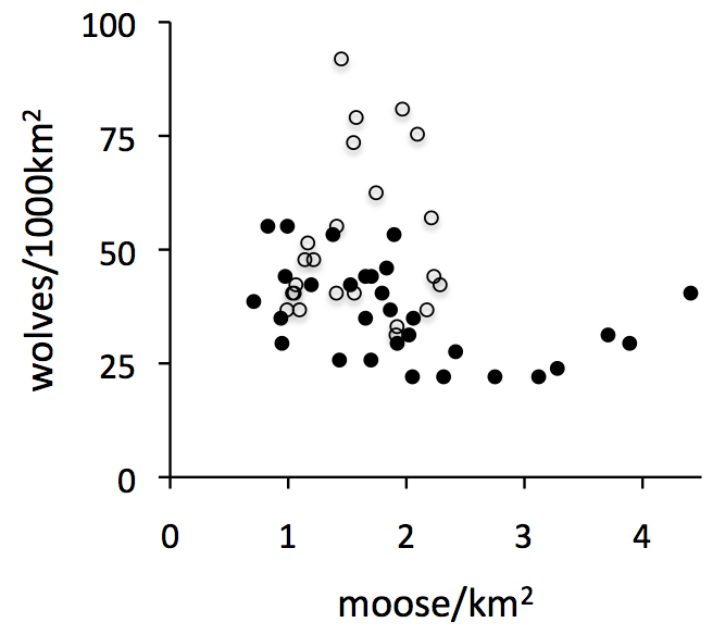
Each symbol on this graph represents the density of moose (read from the horizontal axis) and the density of wolves (read from the vertical axis) for a particular year. The open circles represent years prior to 1980, and the black circles are years after 1980. The year 1980 was an important tipping point in wolf-moose dynamics, triggered by canine parvovirus (Wilmers et al. 2006)[pdf].
Wolf and moose densities are the total number of wolves and moose on Isle Royale, divided by the size of Isle Royale, 544km2. Expressing abundance in terms of density allows us to compare Isle Royale wolf-moose dynamics with those observed in other parts of the world.
This graph tells a great deal about how wolf and moose populations are interconnected. If, for example, wolf abundance was determined primarily by food availability and if total moose abundance indicated food availability, then wolf and moose abundances would be positively related. This kind of relationship is what ecologists refer to as the bottom-up control of a food chain.
By contrast, if moose abundance was determined primarily by wolf predation, and if wolf abundance was a good indication of predation pressure, then wolf and moose abundance would be negatively related. This kind of relationship is what ecologists would refer to as the top-down control of a food chain.
This graph shows that wolf and moose abundances are neither positively nor negatively related. In other words, fluctuations of wolves and moose on Isle Royale are not explained by either simple top-down or bottom-up explanations. The true explanation is quite a bit more complex.
3. How much food does each wolf get?
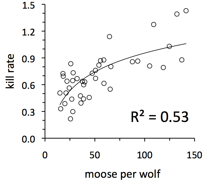
The per capita kill rate (or sometimes just called kill rate) is a special statistic indicating how much food the average wolf in a population gets. The kill rate is calculated by observing how frequently wolves kill moose. More specifically, the kill rate is the number of moose killed, divided by the number of wolves in the population making those kills, divided by the time we spent observing those kill events. Consequently, the units on kill rate are kills per wolf per month. In this graph, the symbols represent the average monthly kill rate for each winter between 1971 and 2011.
The most remarkable observation is just how variable kill rate is. The highest kill rate we ever observed was in 1992. That kill rate was more than twice the average kill rate. The lowest kill rate we ever observed was in 1981. That kill rate was less than a third of a typical kill rate. Imagine an entire winter where you got twice the normal amount of food, or less than a third.
Ecologists have long known that predator kill rates are variable. The challenge has been to understand why. One of the earliest theories, going back nearly a century, is that kill rate should be greatest during years when prey are most abundant, mainly because abundant prey should be easier to find when they are abundant. A more recent idea is that kill rate might also tend to be lower during years when predators are more abundant. Why? One reason is that when predators are more abundant, they might spend more time on activities like defending their territories from other predators.
These two ideas can be combined by supposing that kill rate should be greatest during years when the ratio of moose per wolf in the population is greatest. The graph above suggests that these processes are important on Isle Royale. Notice where the graph says “R2=0.53.” What does that mean? R2 is a statistic that can range from zero to one. A value of one would indicate that fluctuations from one year to the next in the number of moose per wolf (i.e., the horizontal axis) explains perfectly all the fluctuations that we observe in kill rate. A value of zero would indicate that moose per wolf explains none of that fluctuation. In this case, with R2=0.53, we can say that fluctuations from one year to the next in the number of moose per wolf (i.e., the horizontal axis) explains about half (53%) of all the fluctuations that we observe in kill rate. Our challenge is to better understand what accounts for the other half of the fluctuations.
For a more technical treatment of these ideas, see Vucetich et al. 2002 (Ecology 83:3003–3013)[pdf].
4. How does food supply (kill rate) affect the wolf population?
In the previous section we learned a bit about what causes the kill rate to fluctuate from year-to-year. Now we can ask, “What are the consequences of those fluctuations in kill rate?.”
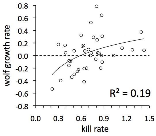
In this graph, each symbol represents a different year for the wolf population. For example, look at the symbol in the lower left portion of the graph. That was the year 1981, when kill rates were the lowest ever and the wolf population crashed from 30 to 14 wolves. That population crash is indicated by how low that observation is, with respect to the vertical axis. Any observation below the dotted line represents a year when the population declined.
More specifically, the vertical axis reflects the percentage by which the wolf population grew each year. For example, in 1977 the wolf population grew from 34 to 40 wolves, an 18% increase or 0.18 growth rate. In that year, the kill rate was 0.30 kills per wolf per month. This observation is far to the left side of the graph and a little high.
Most important is the overall trend revealed by this graph. That trend is for the population to grow more during years when food was more plentiful, i.e., when kill rate was higher. Although this trend is pretty much what you might expect, there is something as subtle as it is important. First, some background: There is a simple, but important idea, that the population dynamics of a top predator should be determined primarily by its food supply. If that were true, then you’d expect the R2 to be much greater than 0.19. This graph shows that most of the variation in wolf growth rate is not explained by variation in food supply.
There are many explanations for what might be going on here, but the list of important factors include disease, inbreeding depression, and demographic stochasticity. For a more technical treatment of these ideas, see Vucetich & Peterson 2004 (Oikos 107:309-320)[pdf].
5. Predation rate, the prey’s perspective on predation.
Predation has two perspectives, the predator’s perspective and the prey’s perspective. The kill rate represents the predator’s perspective on predation. Now let’s consider the prey’s perspective, which is represented by another important statistic, the predation rate.
Predation rate is the proportion of moose each year that are killed by wolves. It is useful to think of a population processes as a balancing act. Predation takes some moose away and the population will decline, unless for example, something like the birth (or recruitment) of new moose offset that loss.
You might think that kill rate and predation rate would be pretty well correlated - that years of high kill rate would tend to be years of high predation rate. You might think that a good year for wolves is a bad year for moose, and vice versa. Turns out that this isn’t the case (see Vucetich et al. [2011], J. Anim. Ecol. 80:1236-1245)[pdf]. Knowing kill rate is only half the story. You also have to investigate the predation rate.
The graph above shows that predation rate has a pretty strong tendency to be greatest during years when moose density (or abundance) is lowest. This trend represents an an important idea. This trend suggests that predation is inversely density-dependent. Here’s what’s going on: Suppose the moose population experiences a series of good years, maybe mild winters or lots of food. Consequently, moose abundance increases and (according to the trend on this graph) predation rate declines. As moose abundance increases, predation becomes a less powerful force, which could allow moose abundance to increase further. Alternatively, suppose the moose population experiences some difficult years and declines, perhaps because of severe winters or lack of forage. As the moose population declines, predation becomes (according to the trend on this graph) an increasingly powerful force, which can cause the population to decline even further.
By this reasoning, predation would be a destabilizing force. We can expect that predation fuels much of the fluctuations we observe in moose abundance. But before we can come to this conclusion, however, we need to consider a few more ideas.
6. How does predation affect the moose population?
This is one of the oldest questions in ecology. The simplest answer is, it depends.
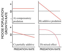
On one hand, predators could focus on prey that would have died anyways - prey that are sick or old. If so, predation doesn’t have much effect at all on prey. Predators would be like scavengers that don’t quite wait for their prey to die. Alternatively, a prey population might respond to increased predation with increased birth rates. In either case, we say predation is compensated by some other process. The result is that increased predation rate has no effect on prey growth rate (panel A). On the other hand, predation could be completely ‘additive,’ where predators are killing prey that would have gone on to live and reproduce had they not been killed. In this case, every one percent increase in predation leads to a one percent decrease in the growth rate of the prey population (panel B).
Other intermediate circumstances are also possible, e.g., where the slope is less steep than negative 1 (panel C) or where predation is compensatory at low rates of predation and increasingly additive at higher rates of predation (panel D).
So how is it on Isle Royale?
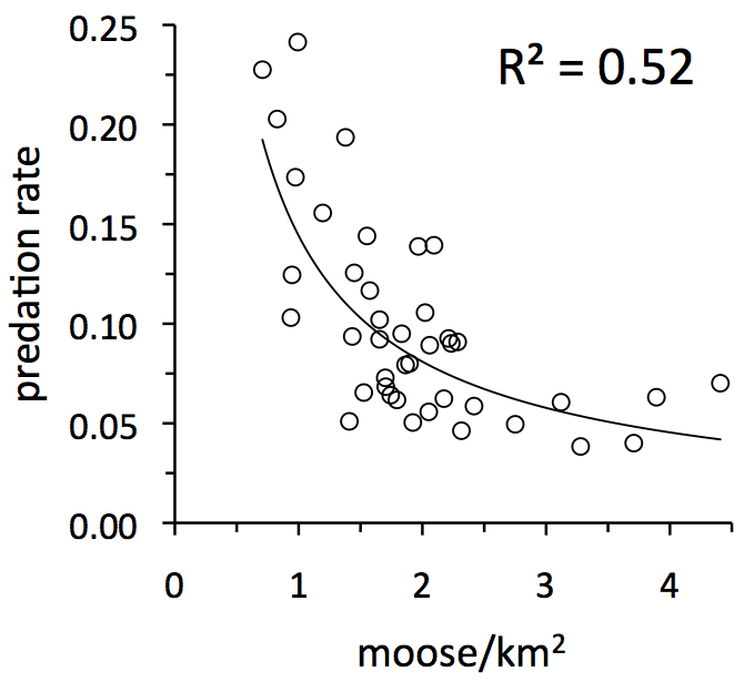
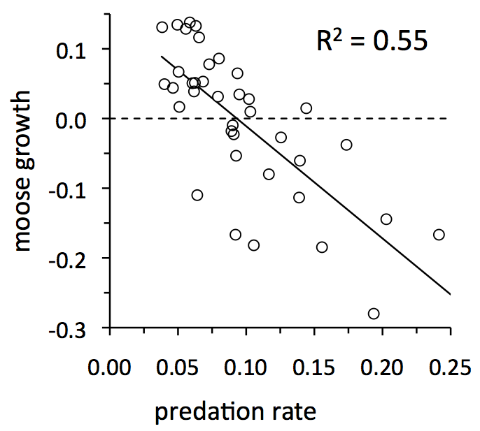
During a typical year on Isle Royale, 1 in 10 moose dies from predation*. In most years, predation rate is between 6% and 13% (see horizontal axis in graph to the left). Overall, predation rate is pretty variable from year-to-year. For example, predation rate is 2 to 4 times greater during years of high predation, compared to years of low predation.
Moreover, predation for Isle Royale moose is strongly additive, with the slope not significantly different from negative one (see graph at left). Consequently, annual variation in predation rate has a big impact on whether the moose abundance will increase or decline. In fact, annual variation in predation rate is one of the most important influences on moose population growth rate (i.e., R2 = 0.55). By the time predation rate exceeds about 10% there is a good chance that the moose population will decline.
*Technical note: On Isle Royale, predation rate is calculated only with respect to moose that have already been “recruited” into the population, or moose that are older than about 7 months of age.
7. Is the moose population unstable, and what does that mean?
So far, it seems that predation rate is an important predictor of whether the moose population will grow or decline (section 6). And, earlier we concluded that predation is a destabilizing force (section 5). These conclusions lead to the question, “Is the Isle Royale moose population unstable?.”
Before answering the question, we need to better understand what it means for a population to be stable or unstable?. All populations fluctuate in abundance. Many of these fluctuations are attributable to ‘environmental stochasticity.‘ For example, environmental stochasticity might be manifest, for example, as a particularly mild winter resulting in high survival, high birth rates and more population growth than would otherwise be expected. Or, for example, environmental stochasticity might, also for example, be manifest as an outbreak of disease, causing an unexpected population decline. A population’s stability determines how a population responds to such perturbations. That is, after a population increases or declines, is there a strong tendency for the population to return to its previous abundance? If so, the population is stable. A population is stable when it tends to return to some long-term average abundance after any environmental perturbation. This kind of stability promotes long-term population persistence. Without this kind of stability a population would grow to infinity (which is impossible), or risk declining to extinction (which is possible).

Stable populations are also said to exhibit density dependent fluctuations. These ideas about stability and density dependence can be represented graphically by a relationship between population density (horizontal axis) and population growth rate (vertical axis).
Consider panel (A). The red line indicates that population growth rate tends to decline with increasing abundance. Moreover, there is a certain level of abundance where growth is zero (red dot). When the population is at this level of abundance the population will not grow or shrink. This is the equilibrium abundance. If environmental stochasticity causes the population to unexpectedly increase from this equilibrium (i.e., move to the right of the red dot), the growth rate in the subsequent year would be negative and the population would tend to decrease, returning to the equilibrium (moving back to the left toward the red dot). 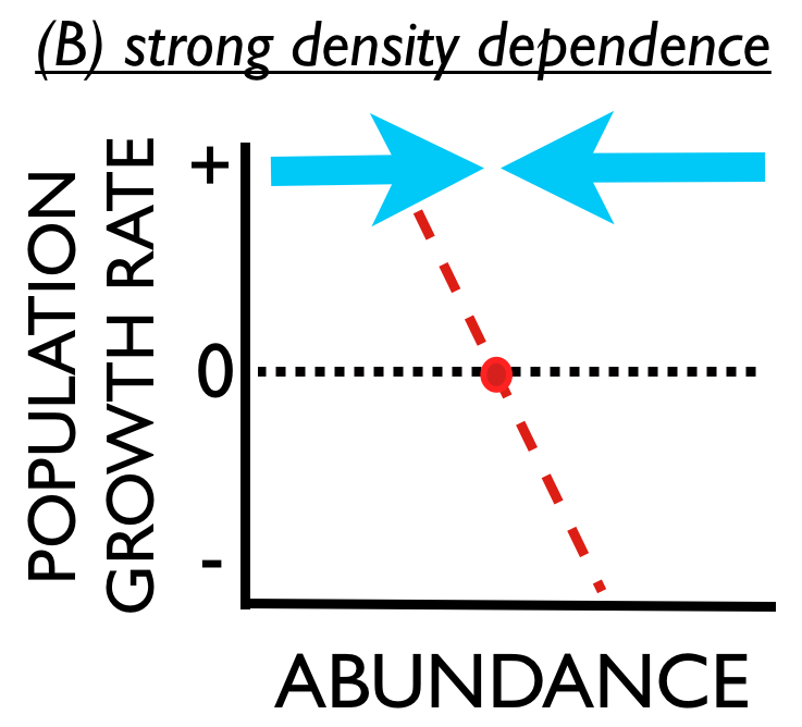 Conversely, if environmental stochasticity causes unexpected population decline, the growth rate in the subsequent year would be positive and the population would tend to increase, again returning to the equilibrium. The population is stable. This stability is also represented by the blue arrows showing how abundance is attracted to the equilibrium.
Any population that persists for any length of time must have density dependence - it is a mathematical consequence of persistence. The more important question is, “How strong is density dependence?.” Panel (B) shows a situation where the red line is much steeper, and the blue arrows are much bigger. This means when a population is perturbed from the equilibrium it will have a very strong tendency to return rather quickly to the equilibrium.
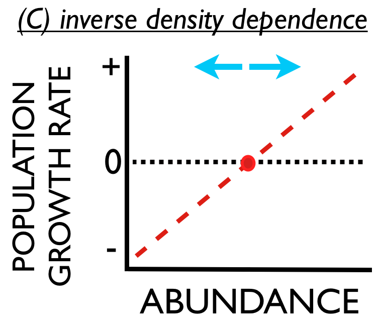
For the broadest context, consider panel (C). Suppose that a population exhibited ‘inverse density dependence,‘ where population growth rate tended to increase with abundance. As before, the population would not tend to increase or decrease when it existed at its equilibrium abundance. However, the population would tend to increase (forever) if some perturbation increased its abundance above the equilibrium. And the population would tend to decline to extinction if some perturbation caused the population to decline below the equilibrium. Such populations are unstable, and may be prone to extinction.
So, how does the Isle Royale moose population compare with these theoretical possibilities? Well, it’s complicated.
For a wide range of moose abundance (i.e., <4 moose per km2), moose growth rate tends to increase with moose density (red dashed line). For this range of abundances, the population is unstable.
But we get a different sense is if we also consider the highest density of moose ever observed on Isle Royale (4.4 moose/km2 in 1996) and the subsequent year when the moose population collapsed (see section 1). 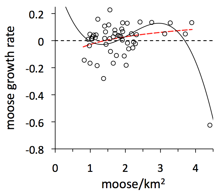 This observation is represented by the point on the lower right portion of the graph. The collapse was caused by a combination of events - most severe winter in a century, outbreak of ticks, lack of forage, and high moose density. When we consider this extreme observation, then the most parsimonious relationship between moose abundance and population growth rate is a complicated curve (3rd order polynomial). That curve indicates the moose population is, overall - across the full range of possible densities - density dependent. That is, the population will tend to increase when abundance is very low and decrease when abundance is very high.
So, while Isle Royale moose are density dependent, in the big picture, they are inversely density dependent, or unstable for a wide range of abundances. This instability is manifest as wide ranging fluctuations in moose abundance (see graph in section 1).
8. Is predation driven by wolves or severe winters?
So far, we know that annual fluctuations in predation rate impact on moose population growth rate (Section 6), predation is a potentially destabilizing force (section 5), and that the moose population is, in fact, quite unstable (section 7).
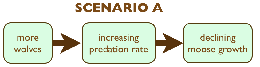
There is one more possibility to assess. Specifically, what causes predation rate to fluctuate from year to year? One might presume it is caused by annual fluctuations in wolf abundance (Scenario A). However, it is possible that severe winters are responsible. Perhaps the direct effect of a severe winter is to weaken the condition of moose, 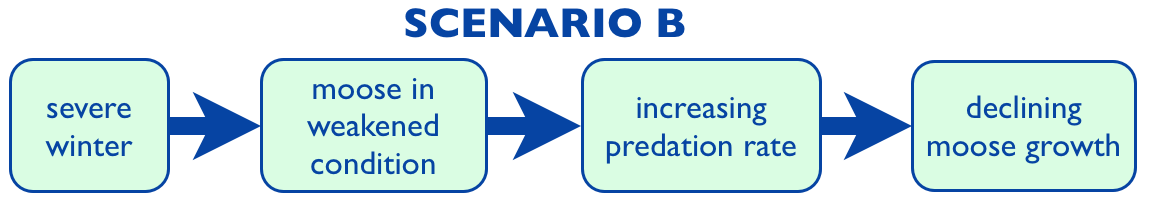 which makes it easier for wolves to kill more moose (Scenario B). In this case, we might say winter weather is the ultimate cause of fluctuating predation rate (i.e., horizontal axis in graphs of section 6), and wolves are only the proximate cause.
We can use data to test whether Isle Royale is more likely characterized by scenario A or B. To do so, we need to compare two graphs - a graph showing how predation rate is related to wolf abundance, and another showing how predation rate is related to winter severity. 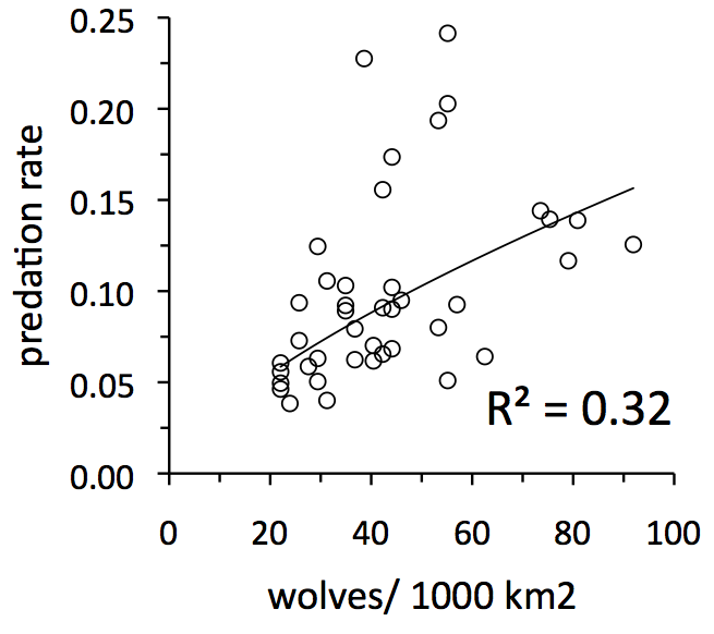 If the predation-rate/wolf-abundance relationship is strong, then we’d conclude that wolves are important in driving predation dynamics on Isle Royale. If the predation-rate/climate relationship is strong, then we’d conclude that predation dynamics on Isle Royale are strongly driven by climate.
The graph to the left shows how wolf abundance has a reasonably important influence on predation rate. Other analyses indicate that 63% of the variation in predation rate can be explained by the number of moose per wolf in the population (Vucetich et al. 2011, J. Anim. Ecol. 80:1236-1245)[pdf].
The next graph requires more explanation. Measuring winter severity is very complicated. Severity depends on the amount of snow, whether 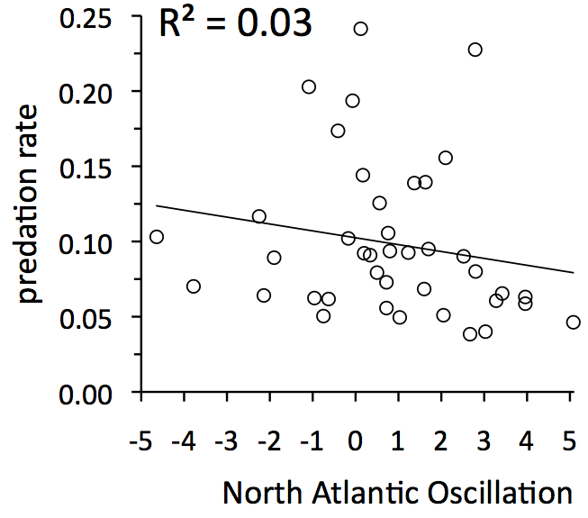 the snow is wet and heavy or light and fluffy, how many months the snow is on the ground, how frequently snow crusts form, etc.
Ecologists have learned that a useful, overall index of winter severity for eastern North America and Western Europe is the North Atlantic Oscillation index. For details on that click here or check out this paper, Ottersen et al. 2001. [Oecologia 128:1-14 DOI]. On Isle Royale, winters tend to be more severe when the North Atlantic Oscillation index is small.
The graph to the left suggests that predation rate has only a slight tendency to be greater during severe winters.
Conclusion: fluctuations in predation rate are drive more by fluctuations in wolf abundance than winter severity.
9. Summing it up, so far
Moose are more than merely a food supply for wolves. Wolves are more than simply a source of mortality for moose. These processes - food for wolves, mortality for moose - are both important, and despite being related to one another, they do not operate in complete synchrony. The result is a complicated set of dynamics. Consequently, the abundance of wolves and moose are not related in any simple manner (Section 2).
For 80 years, predation theory has guided the observations that field ecologists make about the predation in the real world. The center pieces of that theory are the functional response and numerical response. The functional response reveals the extent to which per capita kill rate varies over time as the density of prey varies (Section 3). The numerical response reveals the extent to which the predator abundance increases or decreases as the kill rate (food supply) varies from one year to the next (Section 4). Together, the numerical and functional responses aim to explain the causes and consequences of fluctuation in per capita kill rate. The wolves and moose of Isle Royale show us that these ideas are important, but explain only a limited portion of the dynamics that occur between Isle Royale wolves and moose. Specifically, the functional response explains only about half the fluctuations in kill rate (R2=0.53), and the numerical response explains only about a fifth of the fluctuations in wolf growth rate (R2=0.19).
Kill rate is predation from the predator’s perspective - it’s their food supply. Predation rate is the prey’s perspective on predation. The most important predictor of whether predation rate will be high or low is the abundance of moose (Section 5). Specifically, predation rate tends to be highest when moose are least abundant. That is, predation is inversely density dependent. That makes predation a potentially destabilizing force. Predation is also largely additive (rather than compensatory) with respect to moose growth rate (Section 6). Consequently, the moose population exhibits only very weak density dependence (Section 7). For a wide range of abundances, the moose population is not attracted to any single equilibrium point, but instead is able to fluctuate up and down with each year’s changing circumstances (climate, food, predation, and more). Finally, it seems that fluctuation in wolves from year to year, not winter severity, is the primary ultimate cause of fluctuations in predation rate (Section 8). That is, wolves have an important destabilizing impact on moose population dynamics.
Nevertheless, there is no worry that wolves would drive Isle Royale moose to extinction. If wolves drove moose to particularly low levels of abundance, the wolf population would be at much greater risk of extinction, due to lack of food. If wolves went extinct, the moose population would increase greatly and be governed by a different set of relationships - forage and climate would become the most important determinants of moose abundance.
10. Age structure: what is it and why does it matter?
Predation rate, kill rate, additive predation, stability, the influence of climate... these are only part of the story. The wolves and moose of Isle Royale are also influenced by the age structure of the moose population.
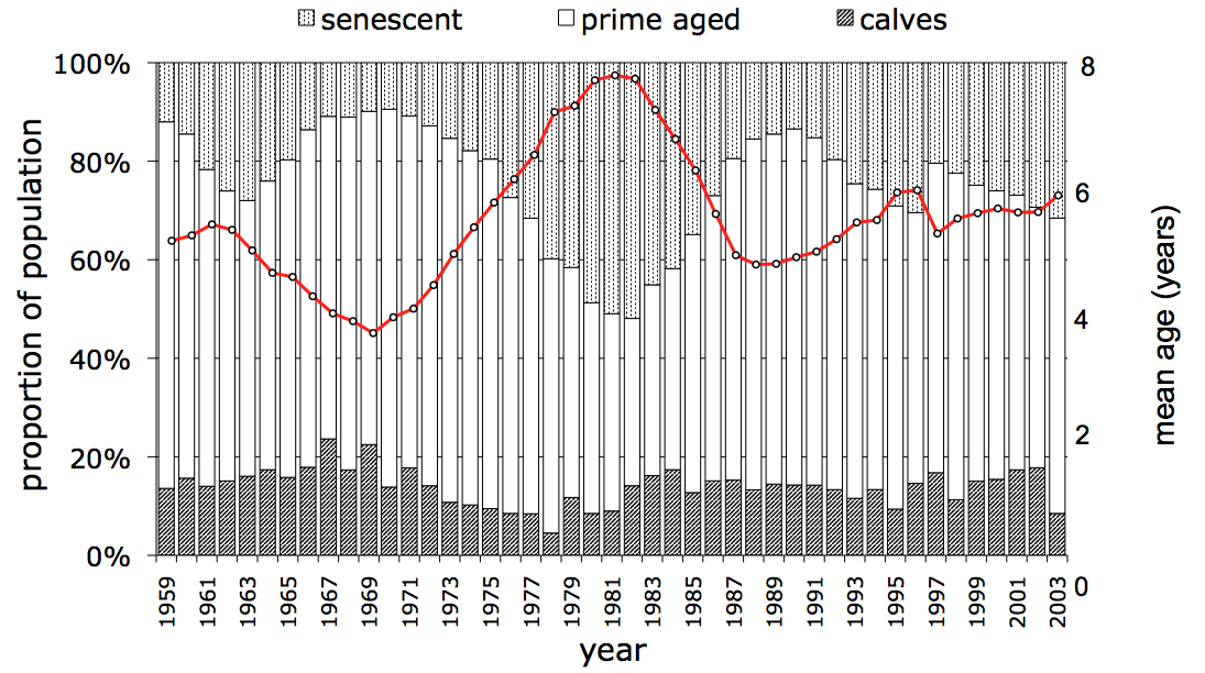
The age structure of a population refers to the proportion of individuals in a population belonging to different age groups. For example, in 1982 primed-aged moose (2-9 years of age) represented about 35% of the population and senescent-aged moose (>9 yrs) about 50%. Over the next decade senescent moose declined to ~14% of the population and primed-age moose had increased to ~65%. These changes are depicted in the graph above.
Each vertical bar in the graph corresponds to a different year. The three portions of each bar, from bottom to top, represent the portion of the moose population that is comprise of calves, prime-aged moose, and senescent-aged moose.
The first important lesson about age structure is that it can fluctuates greatly over time. Another way to describe this fluctuation is by the average age of moose in the population, which has ranged from ~3 years to almost 8 years of age (red line and right axis in graph).
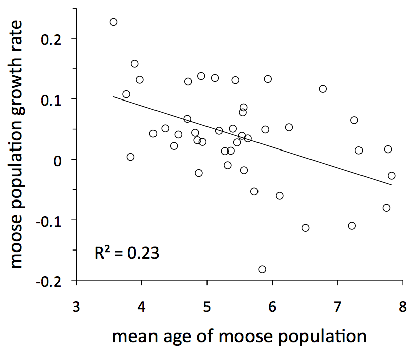
Age structure is important for a second reason. That is, the ecology of an individual varies greatly with its age. Prime-aged moose have the highest rates of survival and reproduction, senescent moose have lower rates of survival and reproduction, and calves have the lowest rate of survival and do not reproduce. These age-specific differences have an important influence on overall moose population dynamics. In particular, population growth rate tends to be lower during years when the average age of a moose is greater (see graph to left). Food might be plentiful, predation might be low, and winter may have been mild. Nevertheless, if the moose population is comprised mostly of very old individuals that are likely to die anyways, then the population might still decline, or at least not increase as much as would otherwise be expected.
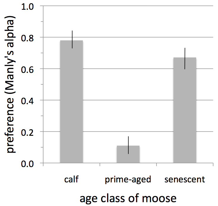
Different-aged moose also exhibit different vulnerabilities to wolf predation. Calves are vulnerable because they are small, and senescent aged moose are vulnerable cause they are often weakened by arthritis, jaw necrosis, or malnutrition. Ecologists describe these differences in vulnerability with a special concept known as preference, which can be quantified by a special statistic, Manly’s alpha. Here’s how preference works: if calves are common in the diet of wolves, it might not reflect wolves’ preference for calves; it might simply indicate that calves are common in the environment. Similarly, if prime-aged moose are rare in the diet, that rarity might not indicate that wolves avoid prime-aged moose, it might simply indicate that prime-aged moose are rare in the environment.
Manly’s alpha helps make this distinction between how frequent a type of food is in the diet, in relationship to how common it is in the environment.
More precisely, if Manly’s alpha equals 0.5 for a particular kind of prey, that means wolves feed on that kind of prey at the same frequency for which it occurs in the environment. Larger values, indicating preference, mean that kind of prey is more common in the diet than would be expected given its frequency in the environment. Values smaller than 0.5 indicate avoidance.
The strongest preference is 1, and the strongest avoidance is 0. For a more technical description of Manly’s alpha see Chesson (1978; Ecology 59:211)[url] and Chesson (1983; Ecology 64:1297)[url].
The graph above was computed from the frequency of each age-class of moose in the environment and in wolves’ diet. Those calculations were made for each year between 1971 and 2003. The three bars represent preference for each age group, averaged across these 32 years. The small vertical lines at the top of each bar represent the standard deviation. These calculations show that wolves avoid prime-aged moose very strongly. It also shows wolves have a slightly higher preference for calves than senescent-aged moose.
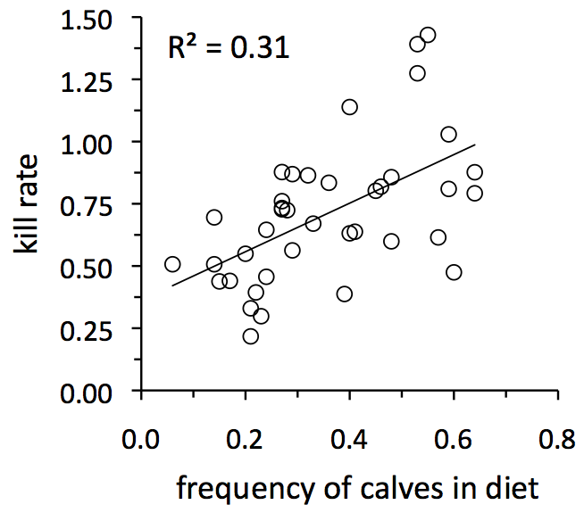
Wolves’ tendency to prefer calves and senescent individuals is a behavior. Behavioral ecology can sometimes seem a world apart from population ecology. However, the two are connected, and ecologists are keen to understand how behaviors affect population processes.
On Isle Royale, per capita kill rate (an important population process) is quite strongly influenced by the frequency of calves in wolves‘ diet, which reflects their behavioral tendency to prefer calves. In years when calves are more common, kill rates are greater. Frequency of calves is the second most important predictor of kill rate (The ratio of moose to wolves is the most important predictor, see section 3). For more, see Sand et al. 2012 (Oikos)[pdf].
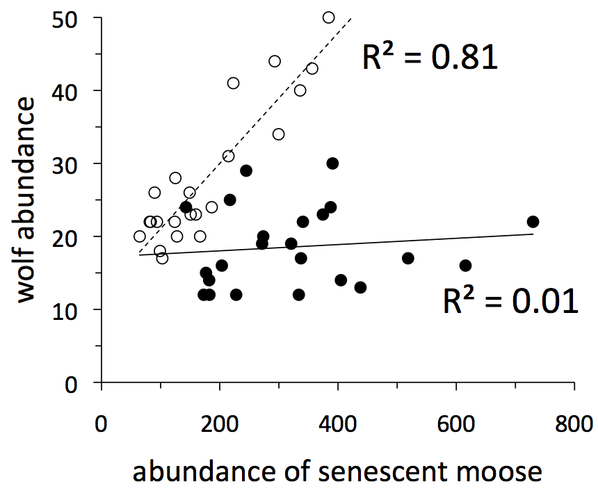
The importance of age structure is manifest in a complex relationship between the abundance of wolves and senescent moose. For the first two decades of observation (1959-1980, open circles in graph to the left), wolf abundance tracked quite closely the number of senescent moose. If the abundance of senescent moose is a good indicator of food availability then the Isle Royale system was strongly bottom-up during those years (see Section 2).
Then, in 1980, the wolf population crashed due to disease (Section 1) and inbreeding took its toll on wolves (see section 12 below). From 1980 onward, Isle Royale shifted from being bottom-up to something else. The abundance of wolves was completely unrelated to the number of senescent moose from 1981-2003.
11. The big shift.
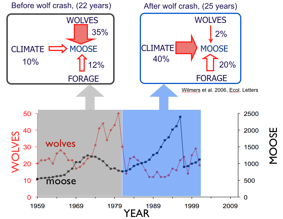
Moose are in the middle of a food chain. They are supported by the abundance of forage below. Wolves represent a pressure from above. And climate is a force that can lead to either increases or declines in population abundance.
Of all the annual fluctuations we observe in the moose population, what portion of those fluctuations can be attributed to fluctuations in wolves, forage, and climate?
For the 22 years between 1959 and 1980, wolves had the greatest influence on moose abundance, and climate and forage abundance were similarly important.
Then for the next two decades, the decades which followed the disease-induced crash of the wolf population, variation in winter severity from year to year replaced wolves as the most important influence on moose population dynamics.
What explains this shift in population dynamics? We consider the most likely explanation in the next section. Quite aside from understanding the cause of this shift, there is an important lesson. After observing the interactions between wolves, moose, and their forage for 20 years, you might think you’d have a reasonably good idea about how those populations worked, especially after getting such a clear answer as we did about the importance of wolves. But then after watching for another 20 years, we got an entirely different answer.
12. Inbreeding depression and genetic rescue in the wolf population.
The Isle Royale wolf population was founded when wolves crossed an ice bridge from Canada in about 1949. They were believed to have been isolated ever since. Comprised typically of just a couple dozen wolves, the population is also small. Small, isolated populations exhibit high rates of inbreeding, which means to mate with close relatives.
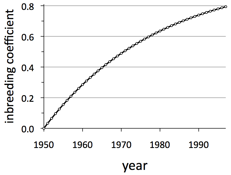
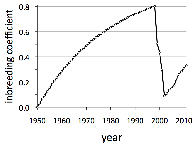
Inbreeding accumulates over the generations, and that accumulation is quantified by the inbreeding coefficient, which is denoted by the symbol F and ranges from zero (completely outbred) to one (completely inbred). Values of F greater than 0.2 frequently cause problems for the health of a population. By the late 1990s, F for Isle Royale wolves had increased to nearly 0.8!
For many decades, the wolves of Isle Royale had been taken as an example of a very small, isolated and highly inbred population which showed no signs of inbreeding depression, the negative impact of inbreeding. But we had it wrong, very wrong. In fact, the population dynamics of Isle Royale wolves have been affected by genetic processes in ways that have been as important as they are subtle.
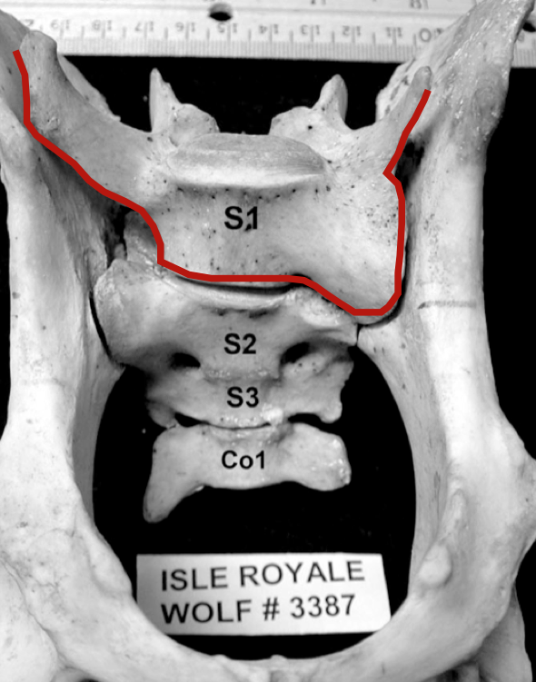
In 2009, with the help of Jannike Räikkönen, an expert in Canid anatomy from the Swedish National Museum, we systematically inspected the skeletal remains from 50, or so, Isle Royale wolves that had been collected over the past five decades. A surprising number of these wolves suffered from several different kinds of congenital malformity in the spine.
Left, is an image of the ventral side of a wolf pelvis and sacral vertebrae. The red line highlights a gross asymmetry. This wolf would have likely suffered damage to nerves that control its tail and hind legs.
A particular kind of deformity, known as a lumbosacral transitional vertebrae (LSTV), is particularly well studied in dogs and wolves. 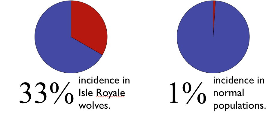 Among healthy, outbred populations LSTV occurs in one out of a 100 wolves. On Isle Royale, a third of the wolves suffered from this malformity.
Not only did Isle Royale wolves exhibit LSTV at a high rate, but the rate of malformities had once been relatively low and increased over the decades, as the population became increasingly inbred. In the graph below, each symbol indicates the year of birth for a different wolf and whether it was born with a spinal malformity (0 = normal; 1 = malformed). The curve represents logistic regression, which predicts the incidence of malformities for each year, based on the observed data. For details, see Räikkönen et al. 2009 (Biol. Conserv. 142:1027-1033)[pdf].
In the 1950s, the expected incidence of malformity was approximately 20%. By the late 1990s, the expected incidence was well over 80%. 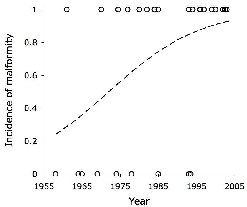 Isle Royale wolves had been suffering from inbreeding depression all along, we just never knew it.
Then something remarkable happened. In 1997 a wolf from Canada walked across the frozen ice bridge that had formed that winter. We had known his identity all along - he was the “old grey guy,” alpha male of Middle Pack during their most successful years. He was physically large and light in the color of his coat (see image below).
Through the analysis of DNA obtained by collecting scat, the “old grey guy” became wolf no. 93. And through that genetic analysis, we learned that no. 93 was not a native Isle Royale wolf, but instead an immigrant from Canada. 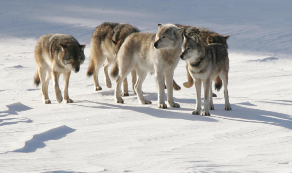 He represented a badly needed infusion of new genes. Within about five years of his arrival, the inbreeding coefficient for Isle Royale wolves dropped well below 0.2 (See graph below).
The fitness of the inbred Isle Royale wolves was so inferior to the fitness of no. 93, that he soon began mating with his own relatives.
He began mating with his daughter in 2002. Over the next several years they produced 21 offspring. Incidences of inbreeding like this caused F to increase again soon after no. 93 arrived.
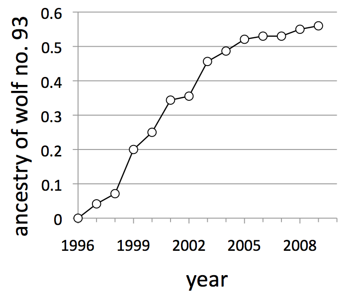
Within a decade of his arrival, 7 of the 8 breeding wolves on Isle Royale were either no. 93 or his immediate offspring. His genes were taking over the entire population.
Ancestry is a statistic indicating the portion of a population’s genome that descended from any particular individual in the population. In large outbred populations, each individual’s ancestry is typically very small. The graph to the left shows how the ancestry of wolf no. 93 steadily grew as he produced more and more offspring and grand offspring. By 2010, more than half the genes in the Isle Royale population were descended from this single immigrant wolf.
So, how has inbreeding and the subsequent genetic rescue affected population dynamics on Isle Royale? A precise understanding is beyond us. However, we have some important general understandings.
First, we have already indicated how the disease-induced population crash of 1980 seemed to trigger an important change in population dynamics for wolves. During the 1980s and early 1990s, wolf abundance never really recovered. Prior to 1980 wolves are an important influence on wolf population dynamics (section 11) and senescent-aged moose were an important predictor of wolf abundance (section 10). However, after 1980, climate replaced wolves as the dominant predictor of moose dynamics, and wolf abundance became completely uncoupled from the abundance of senescent-aged moose. In retrospect, these changes were likely the result, at least in part, of inbreeding depression.
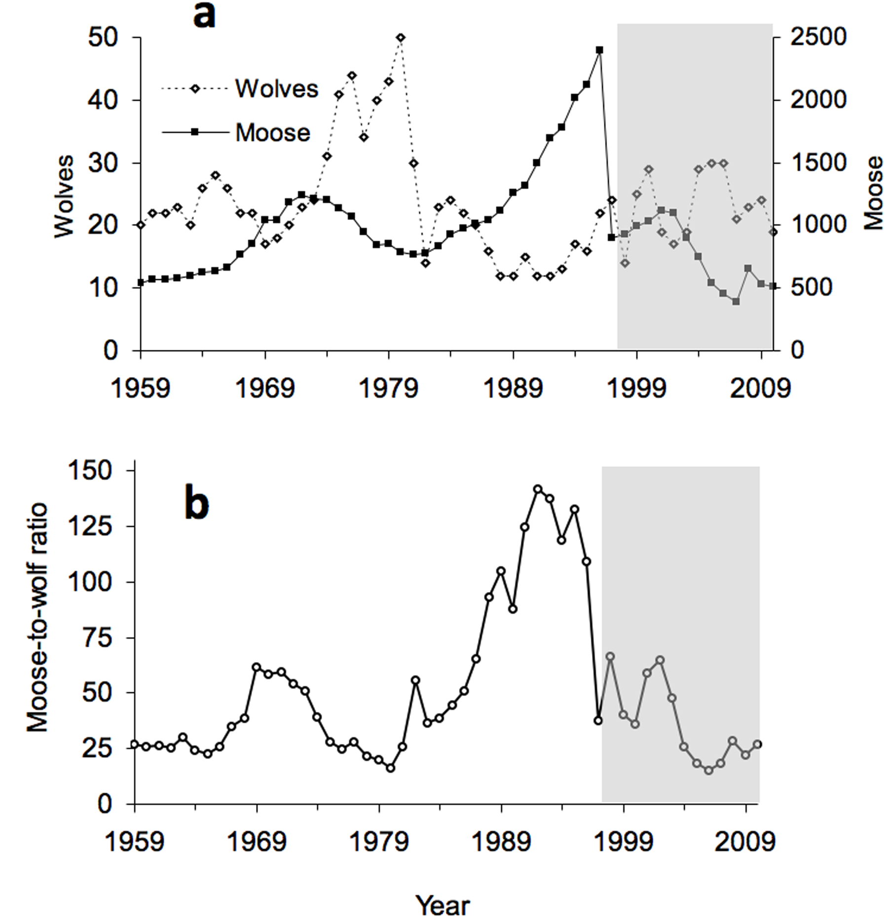
So did wolf demography improve after the immigrant’s arrival? The answer is complicated. After no. 93’s arrival, wolf abundance may have generally increased, but that increase was pretty erratic and not statistically significant (see panel A, to the left). The shaded portions of these graphs highlight the period of time after the arrival of no. 93.
However, the immigrant’s arrival was associated with a time when the number of moose per wolf declined dramatically (shaded area of panel B, at left). Recall that the number of moose per wolf is an important indicator of food availability for wolves (section 3). Given that circumstance, the wolf population should have declined, and probably by quite a bit, at the time when the immigrant arrived. The arrival of wolf no. 93 is almost certainly the reason why the wolf population showed a slight tendency to increase at a time when food was not particularly plentiful. For more about wolf no. 93, see Adams et al. 2011 (Proc. R. Soc. 278, 3336-3344) [pdf].
13. What is calf recruitment declining and why does it matter?

Recruitment rate is the proportion of the moose population that is calves. We measure recruitment rate in mid-winter when calves are 8-9 months old. Knowing the recruitment rate can be more valuable than knowing the birth rate. That is, it may not be so important to know how many calves were born in May, but instead to know how many calves were born and survived their first several months of life.
For populations of moose (and other ungulates), recruitment rates tend to fluctuate greatly, and they are important for understanding how and why moose abundance fluctuates tend to increase. (See graph to the left.)
Recruitment rate has been steadily declining for the past 25 years on Isle Royale, and we don’t know why. 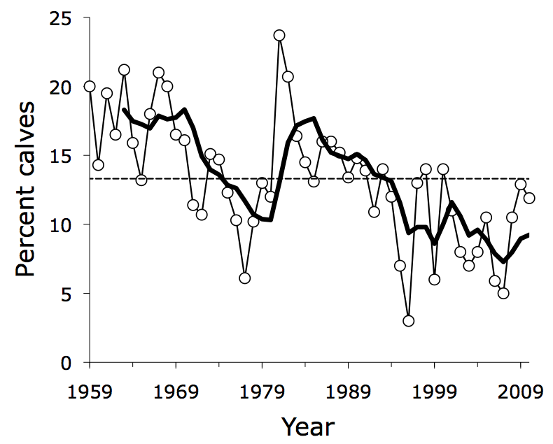 Recent declines in recruitment are also associated with some of the lowest levels of moose abundance ever observed on Isle Royale (see graph in Section 1).
Recruitment tends to be lower when predation rate is higher and moose density is higher. But those influences do not seem to provide an adequate explanation for why recruitment has experienced such a long-term decline.
Climate warming and increased ticks might have something to do with the most recent low levels of recruitment. Forest succession might also explain some of the decline. Ultimately the decline is troubling, and remains unexplained.